Frontier: Elite 2 - Graphics Study

Introduction
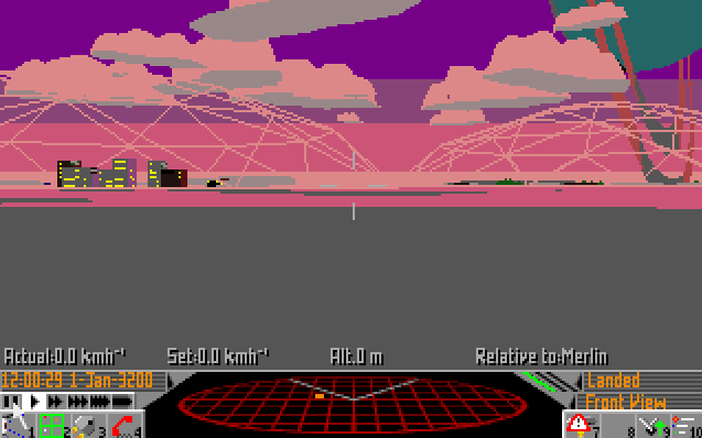
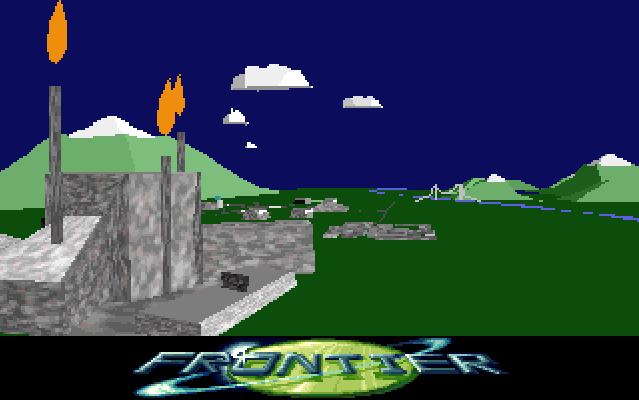
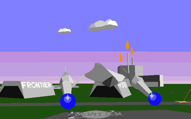
Frontier: Elite 2 (FE2) was released in 1993 on the Amiga by David Braben. The game was an ambitious spaceship sim / open galaxy sandbox, squeezed into a single floppy disk. You could launch your ship from a space station, jump to another star system, travel to a distant planet, land and dock at the local spaceport, fighting pirates and avoiding police along the way.
Planets had atmospheres, rings and surface details. Moons, planets and stars moved across the sky. Any planet in a system could be visited. Any star system in the galaxy could be jumped to. You could even use gravity to slingshot your ship around stars and planets.
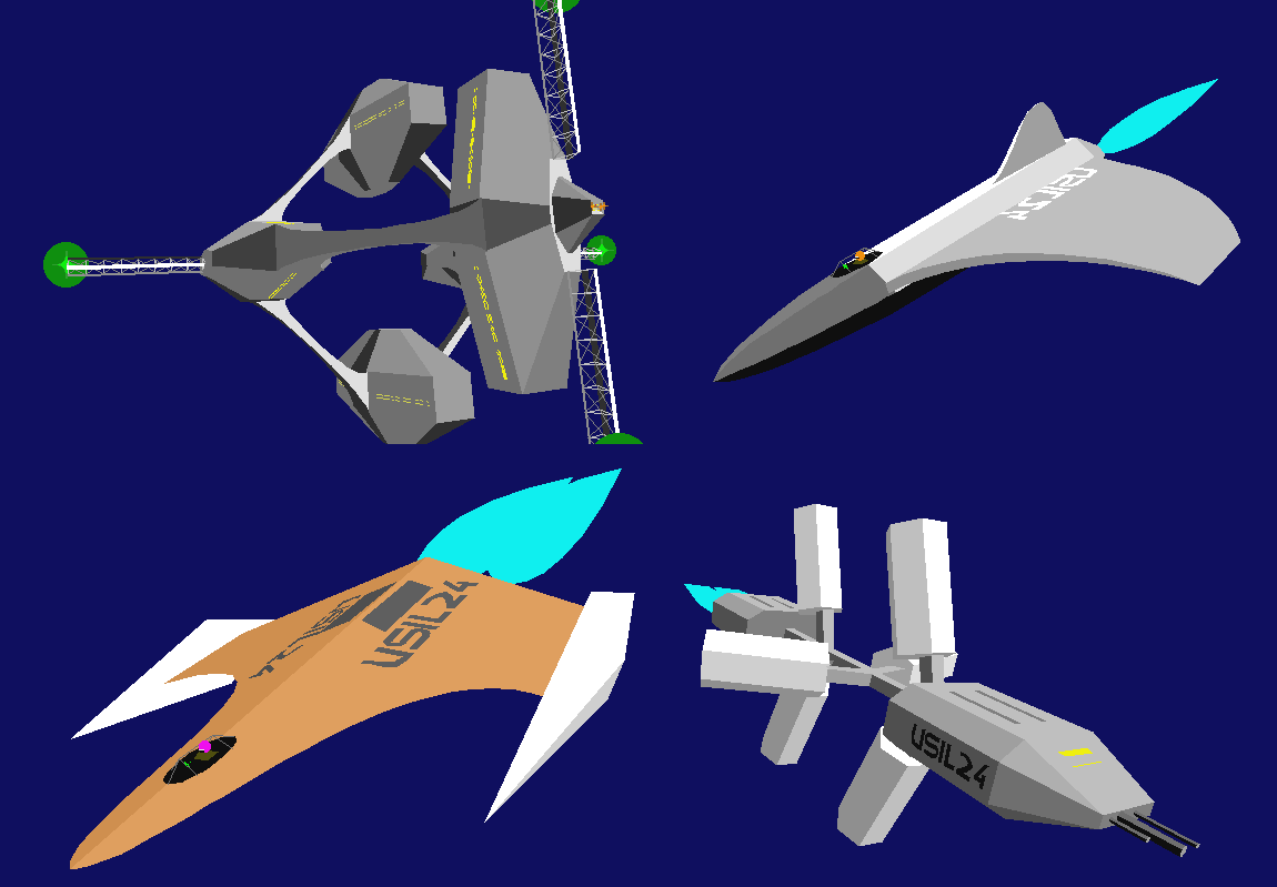
The Frontier 3D engine was tailored for rendering planets, moons, stars, spaceships and habitats on an Amiga. Here are some notable features of the Frontier 3D engine:
- Planetary atmospheres & surface details
- Star System lighting & shading with dynamic palette
- Curved polygons / surfaces
- 3D text
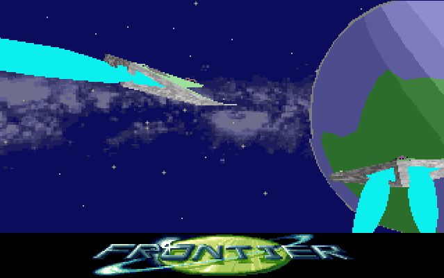
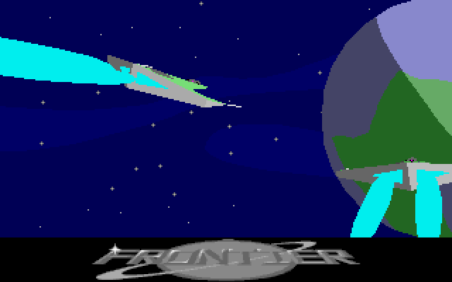
- Engine plume / trails
- Lens flair effects
- Lines and detailing
- Level of Detail (LOD) based on distance
- Huge variety of star / planet / ship / city / starport models
How was it all done? Due to variety of the graphics and jam packed features I was more than a bit bamboozled! Read on to find out more about the graphics side of things. I won't go into the other aspects of the game (much), but you can check out the additional info sections at the bottom if you are curious.
Target Platforms
The target machines were the Amiga and AtariST. A baseline Amiga 500 comes with a Motorola 68000 16-bit 7MHz CPU. The AtariST and Amiga version were released at the same time. At that time the 68K CPU was pretty commonly used, a port to the Mac would have been straight forward.
The resolution targeted was 320 x 200 with up to 16 colours on-screen at any one time. The colour palette was from a possible 4096 colours. The 16 colours were assigned via a 12-bit RGB format: 4 for Red, 4 for Green, 4 for Blue. The 3D scene was rendered in the top 168 rows, the ship cockpit / controls were displayed in the bottom 32 rows (or the case of the intro - the Frontier logo).
The baseline Amiga could support a 32 colour palette, but the AtariST was limited to 16 colours so the engine has to work with just 16 colours available. This may be why the Amiga version is limited to 16 colours as well (also it's one less bit plane to have to draw into).
The PC version came slightly later, and has a few additions over the Amiga version. It was translated to x86 assembly from the 68K assembly by Chris Sawyer. PCs were really Moore's law'ing it up at the time, and FE2 on the PC made good use of the extra horsepower available. The additions are listed below.
Models
Each star / planet / ship / city / starport / building / etc is stored as model with a list of vertices, normals and a list of opcodes. The opcodes encode the lines, triangles, quads, complex polygons to render as part of the model. But the opcodes can do much more than this. Most of the model specific rendering logic is described by the model code. It is used for level of detail (LoD) decisions, model compositions, animations.
Instead of writing assembly code to control how each model is rendered, a model's opcodes are run in a Virtual Machine (VM) with a set of inputs (e.g. time, position, orientation, ship details, pseudo random variables). These are passed in from the code that requested the object to be rendered.
When each object is rendered, its model is looked up and then its opcodes are executed in a VM. These are executed every frame to build a raster list (aka draw list). The raster list contains the list of things to be drawn on screen and where they should be drawn.
As discussed the first few opcodes specify a primitive to render. There are also opcodes for conditional logic, branches and calculations. These are used many creative purposes, chiefly:
- Distance based Level of Detail (LOD)
- Model Variety (Colours, conditional rendering)
- Animations (Landing gear, docking, explosions)
Other opcodes instruct the renderer to render entire 3D objects:
- Planets / Stars
- Spheres
- Cylinders (e.g. Landing gear wheels, courier engines, railings)
- Other models (in a given reference frame)
- 3D text strings
Per Frame Breakdown
On the Amiga, screen clears are done using the Blitter. This happens in the background while the game gets on with updating game logic and deciding what models to render. The models are then rendered, and a raster list consisting of triangles, quads, lines, circles, etc is built. The raster list is stored as a binary tree sorted by z-depth. Once all models are done adding items to the raster list, the game checks that the Blitter is done clearing the screen's backbuffer (which it normally is at this point). Then everything is rendered back to front by traversing the binary tree.
- Kick off a screen clear of back buffer using the Blitter (double buffering)
- Run game update logic, building list of model instances to render
- Iterate through model instances:
- If bounding sphere is outside viewport, skip
- Run model opcodes in the VM, building the 2D raster list as we go
- Once raster list is complete, look at colours used and build a palette
- Wait for Blitter clear to be done
- Build the 16 colour palette
- Raster graphics from back to front, to back buffer
- On vertical blank:
- Flip back buffer and front buffer
- Load new palette to HW
Raster List
The raster list (or draw list) is the list of items to draw on-screen. It is built, each frame, by the 3D renderer. The 3D renderer is invoked for each object, and applies visibility checks, clipping and 3D projections to come up with the list of 2D stuff to draw.
    ; Draw two quads and then a triangle.
    ; The number before the colon is the z-depth.
    1459: QUAD ([295, 200], [317, 234], [337, 287], [291, 213], 4)
    12e7: QUAD ([415, 170], [354, 179], [317, 234], [337, 287], 9)
    12e7: TRI ([83, 34], [354, 179], [317, 234], 9)
The raster list is organised as a binary tree keyed off a depth (Z distance) per raster item. When it comes to actually drawing the list, it can be easily traversed from back to front, so that nearer objects are drawn over those in the background (painter's algorithm). The depth of any given raster item is typically given by one of its vertices, or min / max of all its vertices. The model code has wide control over which method is used.
Sorting all the polygons/raster items every frame is slow, so FE2 has a number of techniques to speed things up.
The binary tree can contain batch nodes, these contain a list of raster items all at the same depth (making insertions after the first item in the batch a simple append). This enforces a raster order for a list of items, one that is independent of the view direction / object rotation. Batches are used to break up large objects into several components, as a speed-up and to help prevent obvious z fighting. Generally you can get away with giving each roughly convex object a single z depth.
In some cases, the batching is ideal, it is used to add extra detail to a polygon without the raster items z fighting. With a modern renderer you would disable the depth test, or bake into a texture / shader.
Another interesting thing is the model code can add sub-tree nodes with their own internal sorting. The whole sub-tree has one z-depth in the outer tree, and any nodes added to the raster list while this sub-tree is active only get added to the sub-tree. This includes depth values that would otherwise be sorted in front of, or behind objects in the outer tree. Frequently used for landing gear, so you don't get any part of the landing gear poking through the main ship model / wing - but, unlike with using a batch, items in the sub-tree remain z sorted.
Any surface with a normal that faces away from the viewer can be skipped by the renderer, so it never gets added to the raster list. In addition, whole objects can be culled if necessary, e.g. missiles under a ship's wing are tied to the wing normal - when the under wing normal faces away from the viewer the missiles are not drawn.
NOTE: One thing to point out here is that even if you had the time to sort every raster item back to front every frame, this won't fully work. You can still have raster items that don't have a 'correct' ordering. Even simple convex objects may not have a canonical Z ordering. The typical example is this: place 3 matchsticks in a triangle, with each matchstick's tip is in front of another matchstick's end - so that stick #1 is in 'front' of stick #2, #2 is in front of #3, which if you follow that logic #3 is in front of #1. Since this is a cycle, there's no way to order it and have it rendered correctly.

So with tight time constraints the best you can do is come up with some compromises that work best for the engine. Later 3D game engines used more expensive techniques like a depth buffer (every pixel is given a depth value) or BSP trees break up polygons so that they do have a canonical sort order).
Lighting
Lighting in-game is directional and coloured from the main star. Each object rendered can have its light source direction & colour setup independently. This is so the light direction is correct for each model when the star is placed near or in the scene, e.g. the orrery view or viewing multiple distant planets.
In the intro and ship view screen the light source is fixed and comes from the top-right of the screen, i.e. above the subject and to the side, much like a standard lighting setup used in cinema.
In most places where a colour is specified, two special bits of the colour are used to indicate how lighting should be applied.
The 12-bit colour format expected by the HW is as follows:
  | Colour | Red  | Green | Blue |
  | Bits   | ba98 | 7654  | 3210 |
But in FE2 when a colour is specified, one bit from each colour has a special meaning:
- Bit 8 - If set emit colour directly / don't add in a normal colour
- Bit 4 - Add the scene base colour (sometimes diffuse, sometimes just object instance colour)
- Bit 0 - This bit is not used, typically the model OpCode borrows this bit for its own purposes
The colour per bit layout is as follows:
  | Red | !Shade | Green | Add Global Colour | Blue | Unused |
  | ba9 | 8      | 765   | 4                 | 321  | 0      |
The computed normal colour (directional light from the star) and global (diffuse) are added directly to the base colour. Since the object colour can only be specified at half intensity, the rest of the colour contribution comes from the global diffuse colour and / or the normal colours.
The set of normal colours to blend (add) are setup with each new reference frame. Colours are either copied form the parent model, or passed in from the code that started rendering the model).
The normal colours and global colour could be overridden by the model code for sub-models, this allowed for additional lights in the scene (albeit one at a time). E.g. hazard lights on space stations and ground control.
Matrix Setup
Rotations were done with a 3x3 fixed point matrix. Since with rotation matrices all the values of the matrix are between -1 and 1, each value could be represented as a signed 16-bit integer implicitly divided by 0x8000, i.e. 0x8000 is -1 and 0x7FFF is ~1.
A scale is built into each model & object, and applied directly on the vertices using bit shifts (the shifting can be cancelled out if needed, say you are rendering an extremely large object from far away).
Offsets / translations are done with separate 3D vectors, and rotated as needed.
When projecting vertices:
- First, the vertex data is read from memory & unpacked
- Second, it is rotated to view space using the current 3x3 rotation matrix
- Third, it is scaled with the current object scale (by bit shifting)
- Forth, it is offset by the current view space object vector
- Finally, it is 3d projected onto the screen - using bit shifts and a depth lookup table (the perspective depth division)
This is done lazily on a per-vertex basis only when the vertex is requested by the model code. This is because A) not all vertices are rendered, since the model code contains conditionals (e.g. LoD) and B) vertices can be dynamically positioned by model code.
Palette Fitting
Two separate palettes are used, one for the 3D area (top 168 rows) and one for the ship cockpit UI (bottom 32 rows), each with 16 colours. The palette is adjusted by a vertical blank interrupt (for the top part) and a copper interrupt (for the bottom part). Note that this is done based on the beam position, so it is independent of the 3D frame render loop, at a constant 50 times per second.
The colour space is 12-bit for a total of 4096 colours, but only 16 of these can be used at any one time. A clever scheme is used to get the most out of these 16 colours. A virtual palette with space for up to 62 colours is created. As new colours are requested by the renderer, they are recorded in the virtual palette. Items added to the draw list reference these virtual colour indexes. Later these will be resolved to real HW palette entries. An array of 4096 slots is used to keep track of which virtual colours are used so far in a frame. At each point in the array, allocated colours marked with their virtual index and unassigned colours are set to with 0 for.
2 fixed colours are always assigned:
- Palette index 14 is always set to the background colour. In space this is #005 (the famous blue space!). On a planet this is set to the colour of the sky. It's fixed because changing the background colour between frames would be a bit too jarring.
- Palette index 15 is always set to gray (#aaa). Used for bitmap text.
So this leaves us with 14 (16 total - 2 fixed) entries to decide on. If there are 14 or less virtual colours, then we are done - the virtual colours can be assigned to the palette directly.
If we've more than 14 colours, well, now some magic needs to happen! The virtual colours need to be merged to fit into the 14 available palette entries. This is done by recursively splitting / partitioning the assigned virtual colours into 14 sBuddyFreeBucketHeads (kinda like quicksort).
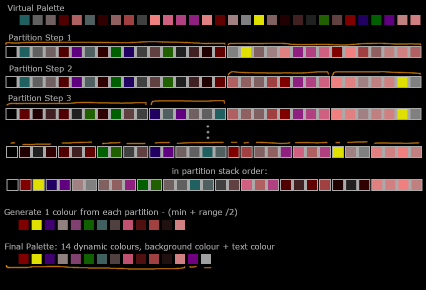
Each partition splits based on the largest color component difference. For example, if the red range is greatest in partition (P1), compared to RGB ranges in other partitions, the red midpoint is used to partition P1 into two partitions. This is done repeatedly - recursively splitting the virtual colours into ranges until we've a total of 14 ranges.
The size of each range at this point is variable, but, normally there will be a small number of colours in the range, e.g. 1-4 colours. At the end of this process, each partition is resolved to a single colour by picking the colour in the midpoint of the partition's colour range (by each colour component). Finally, these colours are stored to be picked up later by the HW on the next double buffer swap.
The PC version has a bigger palette to work with and doesn't use this colour matching scheme. It has more colour palette entries available than even the virtual colour list on the Amiga version. As such, it rarely needs to do any colour merging / palette compression at all. This is the version I've implemented.
Scale and Numeric Precision
The 68K processor could only do 16-bit multiplies and divides, and each took many cycles to complete (MULS - Multiply Signed: took 70 cycles, DIVS - Divide Signed - took a whooping 158 cycles, compare this to add / subtract which took around 6 cycles). Hardware supported floating point was very rare as it required an upgraded or expensive Amiga. Not much software supported HW floating point and for real time 3D it often wasn't faster than a fixed point scheme anyway (as much of the precision is unneeded / can be worked around). Anyway, end result, the Frontier engine implemented its own fixed point & floating point code using integer instructions.
There are two schemes used (in the renderer):
- Fixed point with a variable for the current scale. This is used by the majority of model code, for transforming vertices and normals, and doing any calculations needed.
- Full software based floating point. This is used by the planet renderer.
There are lookup tables & supporting code for many operations:
- Perspective divide (with near clipping built-in to lookup data)
- Sine and cosine
- Square root for calculating distance / vector length
- Arctan
Two software floating point number sizes are supported:
- 32-bit: 15 bits for mantissa (factional part), 16 bits for exponent (embiginess part), 1 bit sign
- 48-bit: 31 bits for mantissa, 16 bits for exponent, 1 bit sign
Note that's a lot of bits for the exponent allowing for some very large numbers (that's not 15 bit shifts, its 32K bit shifts!). This is mainly due to it being easier this way since it is implemented with 16-bit integer math primitives. Compare the exponent size to IEEE floating point 754, which uses only 11 bits for the exponent in 64-bit floating point!
Planet Rendering
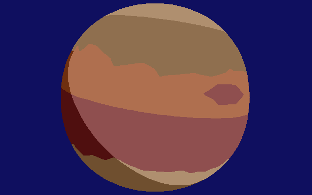
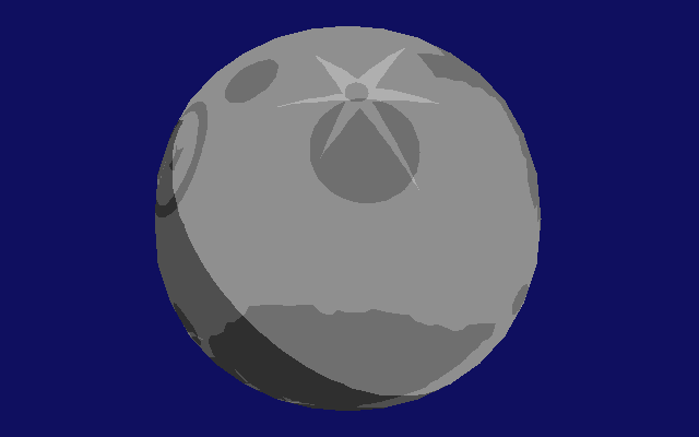
The planet renderer is very special, it has its own raster list primitives, uses its own floating point number scheme, and is mostly custom code vs being rendered using existing model opcodes.
There are three types of surface features:
- Surface polygons - Land masses on earth-likes, or colour bands on jupiter-likes
- Surface circles - Polar ice caps
- Shading in the form of 1 - 3 arcs (these typically cut across the other surface features)
The surface polygons are mapped to the surface of the planet by treating them as arcs across the surface. Procedural sub-division of the surface polygon line segments are used to add surface detail as you get closer to the planet.
A set of atmospheric colours can be specified, these are rendered when looking at a planet / star side on.
Which brings us to the view dependant rendering paths:
- When the planet covers most of the screen the background colour is changed to the sky or ground colour to avoid overdraw.
- When the planet is at the edge of the screen, or you were viewing along the surface, the outline is rendered with a single Bézier curve. Any atmospheric bands are rendered with additional Bézier curves.
- When the planet outline covers enough of the screen to be elliptical, it is rendered with two Bézier curves.
When it comes to rasterising the planet, a custom multi-colour span renderer is used. The renderer generates an outline of the planet, then adds surface details, and finally arcs for shading are applied on top. This generates a set of colour flips / colour changes per span line within an overall outline, which are sent to the rasteriser.
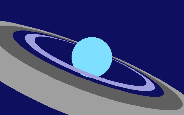
Planets rings are implemented in model code, using the complex polygon span renderer (Bézier curves strike again!).

How are weather pattern effects done? You guessed it! Using Bézier curves & the complex polygon span renderer.
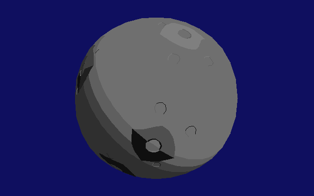
Ditto for craters on moons / smaller planets.
Model Data
Each model in the game has the same basic model structure:
- Code offset, #vertices, #normals
- Scale and bounding sphere
- Base colour
- List of vertices
- List of normals
- Model OpCodes to be executed per frame
Example Model
Frontier renders the 3D world using its own OpCodes / bytecode (well actually 16-bit wordcode, because it was written with 16-bit buses in mind). This code specifies the primitives to display, level of detail calculations, animations, variation and more.
The original source code was written directly in assembly. The model code was likely directly typed in as data blocks in the assembly files. Most instructions and data align to 4, 8, 12 or 16 bits which is perfect for just typing in the hex values (which is 4 bits per character, i.e. 0x7002 0x0102 - draws a red (0x700) line (opcode 0x2) from vertex 1 (0x01) to vertex 2 (0x02)).
To easily read the model code without documenting every line, I added code to convert it to an intermediate text format. This syntax is completely made up by me on the spot and not part of the original game.
Here's an example model, you'll learn about the details in the following sections.

; Single polygon heart logo
; Commented lines start with ;
; Actual compiled words are commented on right
model: 3                      ;   0032 - codeOffset
  scale1: 16,                 ;   001e - vertexDataOffset
  scale2: 0,                  ;   0100 - verticesDataSize * 64
  radius: 40,                 ;   002e - normalsOffset
  colour: #04c                ;   0008 - normalDataSize + 4
                              ;   0010 - ^2 scale
                              ;   0000 - unknown
                              ;   0028 - radius
                              ;   0000 - unknown
                              ;   004c - colour
                              ;   0000:0000      - unknown
                              ;   0000:0000:0000 - unknown

vertices: ; 4                 ;
  0, -15, 0                   ;   0100:f100 - vertex index 0
  0, 30, 0                    ;   0100:1e00 - vertex index 2
  25, -35, 0                  ;   0119:dd00 - vertex index 4
  45, -13, 0                  ;   012d:f300 - vertex index 6

normals: ; 1
  0 (0, 0, -127)              ;   0000:0081 - normal index 2
                              ;   placed at vertex 0
                              ;   length should always be 127

code:
  complex normal:2 colour:#800 loc:end  ; 8005:0c02
  cbezier 0, 4, 6, 2                    ; 0200:0004:0602
  cbezierc 7, 5, 0                      ; 0807:0500
  cdone                                 ; 0000
  end: done                             ; 0000
Vertex Encoding
Each vertex is specified in 32 bits:
- 1 byte for vertex type
- 3 bytes of information specific to the vertex type
The vertex type controls how the vertex is computed and projected.
For the base vertex type the 3 bytes encode the signed (X, Y, Z) values for the vertex. For the other vertex types these bytes can refer to other vertices, or even model code registers.
The different vertex types are:
| Hex# | Vertex Type | Params | Description |
|---|---|---|---|
| 00, 01, 02 | Regular | X, Y, Z | Regular vertex with X, Y, Z directly specified |
| 03, 04 | Screen-space Average | Vertex Index 1, Vertex Index 2 | Take screen-space average of two other vertices |
| 05, 06 | Negative | Vertex Index | Negative of another vertex |
| 07, 08 | Random | Vertex Index, Scale | Add random vector of given size to vertex |
| 09, 0A | Regular | X, Y, Z | Regular vertex with X,Y,Z directly specified |
| 0B, 0C | Average | Vertex Index 1, Vertex Index 2 | Average of two vertices |
| 0D, 0E | Screen-space Average | Vertex Index 1, Vertex Index 2 | Take screen-space average of two other vertices, but don't project sibling vertex |
| 0F, 10 | AddSub | Vertex Index 1, Vertex Index 2, Vertex Index 3 | Add two vertices, subtract a 3rd |
| 11, 12 | Add | Vertex Index 1, Vertex Index 2 | Add two vertices |
| 13, 14 | Lerp | Vertex Index 1, Vertex Index 2, Register | Lerp of two vertices, as specified by model code register |
When vertices are referenced by model code, negative numbers reference vertices in the parent model. Indexes are multiplied by 2, with even numbered indexes referencing vertexes specified in the current model as is, and odd numbers referencing the same vertices but with the x-axis sign flipped.
The parent model can choose what (0-4) vertices to export to sub-models, this is done as part of the 'MODEL' opcode.
A vertex index in model code is stored as 8-bits, with only positive vertices from the current model, and a bit for flipping the x-axis, this resulted in a total of 63 possible vertices per model / sub-model.
Vertices are projected on demand, if a vertex is not referenced by the model (or is skipped over due to LOD tests / animations) it is not transformed / projected. The Lerp vertex type essentially requires that vertices be projected on demand, as it examines the VM scratch registers while the model opcodes are running. This process is recursive, so if vertex A references vertex B, which references C, C has to be transformed first, then B, then finally A. As an optimization sometimes a vertex and its pair (the neg X-axis version of the vertex) will be transformed at the same time.
Normal Encoding
Normals are also encoded in 32-bits:
- 1 byte for the vertex index this normal applies to (used for visibility checks)
- 1 byte for X
- 1 byte for Y
- 1 byte for Z
A normal index in model code is stored as 8-bits, and one of these bits (LSB) flips the x-axis. 0 typically specifies no normal. This results in a total of 126 possible normals specified per model / sub-model.
When normals are referenced by index, to get the real index divide by 2 and subtract 1. So 2 would be the first normal specified in the model, 3 is the same normal but x-axis flipped, 4 is the second normal, and so on.
Model Code
Instructions vary in the number of words they take up, but the first word always contains the opcode in the 5 least significant bits. Often the colour is stored in the remaining part of the word.
Here's a full list of the opcodes and what they do:
| # | Hex# | Opcode | Description |
|---|---|---|---|
| 0 | 00 | DONE | Exit this models rendering |
| 1 | 01 | CIRCLE | Add circle, highlight or sphere to draw list |
| 2 | 02 | LINE | Add line to draw list |
| 3 | 03 | TRI | Add triangle to draw list |
| 4 | 04 | QUAD | Add quad to draw list |
| 5 | 05 | COMPLEX | Add complex polygon to draw list |
| 6 | 06 | BATCH | Start / end a draw list batch (all items in the batch have same Z value) |
| 7 | 07 | MIRRORED_TRI | Add a triangle and its x-axis mirror to draw list |
| 8 | 08 | MIRRORED_QUAD | Add a quad and its x-axis mirror to draw list |
| 9 | 09 | TEARDROP | Calculate Bézier curves for engine plume and add to draw list |
| 10 | 0A | VTEXT | Add vector text (3D but flat) to draw list |
| 11 | 0B | IF | Conditional jump |
| 12 | 0C | IF_NOT | Conditional jump |
| 13 | 0D | CALC_A | Apply calculation from group A |
| 14 | 0E | MODEL | Render another model given a reference frame |
| 15 | 0F | AUDIO_CUE | Trigger an audio sample based on distance from viewer |
| 16 | 10 | CYLINDER | Draw a cylinder (one end can be bigger than other so really it's a right angle truncated cone) |
| 17 | 11 | CYLINDER_COLOUR_CAP | Draw a capped cylinder |
| 18 | 12 | BITMAP_TEXT | Add bitmap text to draw list |
| 19 | 13 | IF_NOT_VAR | Conditional jump on variable |
| 20 | 14 | IF_VAR | Conditional jump on variable |
| 21 | 15 | ZTREE_PUSH_POP | Push / pop sub ztree |
| 22 | 16 | LINE_BEZIER | Add Bézier line to draw list |
| 23 | 17 | IF_SCREENSPACE_DIST | Jump if two vertices are within / past a certain distance in screen coordinates |
| 24 | 18 | CIRCLES | Add multiple circles / spheres / stars to draw list |
| 25 | 19 | MATRIX_SETUP | Setup tmp matrix, either rotate given axis away from light source or set to identity |
| 26 | 1A | COLOUR | Set base colour (added to all colours), or directly set a normals colour tint |
| 27 | 1B | MODEL_SCALE | Render sub-model with change of scale |
| 28 | 1C | MATRIX_TRANSFORM | Transform tmp matrix using rotation about axis and axis flips |
| 29 | 1D | CALC_B | Apply calculation from group B |
| 30 | 1E | MATRIX_COPY | Overwrite model view matrix with tmp matrix |
| 31 | 1F | PLANET | Astronomical body renderer w/ surface details and halo / atmosphere effects |
This model code text can be compiled into the original model code - which allows making modifications / trying different things out. This all adds a lot of complexity, so I've put it in its own set of optional files modelcode.h and modelcode.c.
Calculations (CALC_A & CALC_B)
The calculation opcodes write to a set of 8 16-bit temporary registers. These can be read as inputs to various other commands e.g. IF_VAR, IF_NOT_VAR, COLOUR and also can be used to calculate vertex positions.
The calculation opcodes can read two 16-bit variables from:
- the 8 16-bit temporary registers
- the 64 16-bit inputs as defined by the calling code to the model renderer
- a small constant (0-63)
- a large constant (0-63 * 1024)
The object inputs are things like the tick #, time of day, date, landing time, object instance id, equipped mines / missiles, etc.
The list of available operations is as follows:
| # | Hex# | Group | OpCode | Description |
|---|---|---|---|---|
| 00 | 0 | A | Add | Add two variables and write to output |
| 01 | 1 | A | Subtract | Subtract one variable from another and write to output |
| 02 | 2 | A | Multiply | Multiple two variables and write to output |
| 03 | 3 | A | Divide | Divide one variable by another and write to output |
| 04 | 4 | A | DivPower2 | Unsigned divide by a given power of two |
| 05 | 5 | A | MultPower2 | Multiply by a given power of two |
| 06 | 6 | A | Max | Select the max of two variables |
| 07 | 7 | A | Min | Select the minimum of two variables |
| 08 | 8 | B | Mult2 | Second multiple command (one is probably signed other unsigned) |
| 09 | 9 | B | DivPower2Signed | Signed divide by a power of two |
| 10 | A | B | GetModelVar | Read model variable given by offset1 + offset2 |
| 11 | B | B | ZeroIfGreater | Copy first variable or 0 if greater than variable 2 |
| 12 | C | B | ZeroIfLess | Copy first variable or 0 if less than variable 2 |
| 13 | D | B | MultSine | From 16-bit rotation calculate sine and multiply by another input variable |
| 14 | E | B | MultCos | From 16-bit rotation calculate cosine and multiply by another input variable |
| 15 | F | B | And | Binary AND of two variables |
Complex Polygon Renderer
When a complex polygon is specified, there's a specialized set of sub-codes for drawing each edge / curve. These can have any number of points, be concave and contain curved edges. The Frontier planet logo at the beginning of the intro and the vectorized 3D text are rendered with these sub-codes.
| # | OpCode | Description |
|---|---|---|
| 00 | Done | Finished complex polygon! |
| 01 | Bezier | Draw a curve given 4 vertices |
| 02 | Line | Draw a line given 2 vertices |
| 03 | LineCont | Draw a line from last vertex to the given vertex |
| 04 | BezierCont | Draw a curve starting at last vertex given 3 new vertices |
| 05 | LineJoin | Draw line from the last point to the first point |
| 06 | Circle | Draw a projected circle as two joined Bézier curves |
The renderer just transforms the vertices, and adds lines / Béziers to the draw list. When the curves get rasterised into lines later they are not perspective corrected, only the end points and the control points are projected. During rasterisation the curves are subdivided into lines in screenspace. This usually looks fine, it's only when a polygon is at an extreme angle to the view plane (changing Z depth over its surface) that you notice warping.
PC Version
The PC version rendered at the same resolution as the Amiga version (320x200) but with 256 colours instead of 16. This was done in 'Mode 13h' with a byte per pixel, i.e. 'chunky' and not bit plane graphics. Colours were still assigned in 4-bit Red, 4-bit Green, 4-bit Blue (i.e. 12-bit colour, for a total of 4096 possible colours). Instead of using the Blitter, the screen clear was done via the CPU writing the background colour index to the screen back buffer. With chunky graphics the rasterizer could be simplified, pixels could be written directly without the need for bitwise composition operations.
Since there's no Copper to change the palette mid-frame, the 256 colors have to cover both the UI and 3D parts of the display, so the palette was split with 128 colours for each.
With way more palette colours available than the Amiga version, a new colour matching scheme was implemented. Also, changing the colour palette on the PC was slow, so the number of colour changes between frames should be minimised. A reference counting / garbage collection mechanism was employed, to keep track of colours between frames. This is the version actually used in the remake.
Another big change was texture mapping. The background star-field was replaced with a texture of the galaxy added to a skybox. Many ships were given textures for extra detailing. The texture maps were fixed to 64x64 texels. But I still preferred the look of the Amiga version, especially at 2x / 4x resolution! Memberries, mayhaps...
Remake Updates GitHub
When converting the renderer to C, I couldn't help but fix a few bugs / add a couple of minor quality improvements. But I tried to be true to the original version, and not change the overall feel or look of the engine.
- 2x and 4x resolution modes
- Clipping fixes for curved surfaces, circles, and complex polygons
- Cylinder render fixes - e.g. courier engines not rendering correctly at some angles
- RTG support for Amiga: 256 colours (like PC version)
- Liberal use of integer divides (unlike any version)
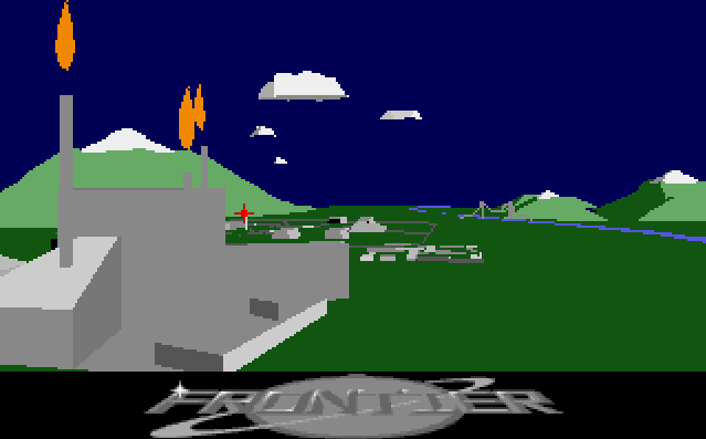
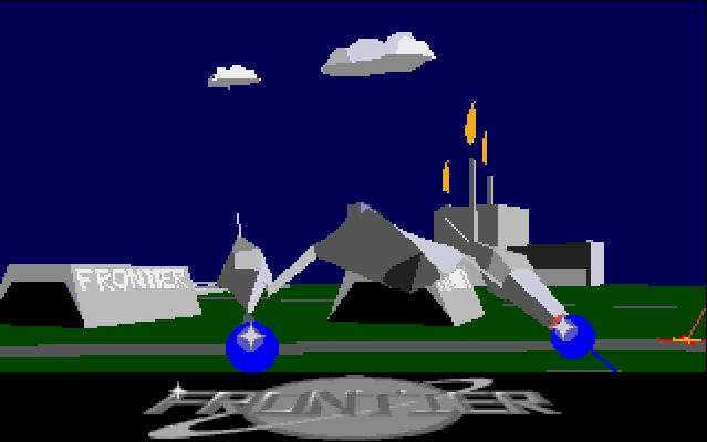
Here's the same screenshot as above but from the original:
Reverse Engineering
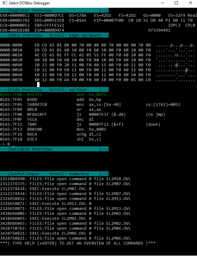
I started with the PC version, mainly as way to learn the ins and outs of x86 DOS coding, plus it was possible to use the free version of IDA to disassemble and annotate the assembly code.
It's important to say there's nothing too special about reverse engineering some code, it's like programming on someone else's project, but you get to stop after the part where you try to understand the existing code :) We are all guilty of skipping the understanding part at some point, but when reverse engineering that's literally the entire job, so we are forced to do it, its good practice I think. Doing this for assembly is like a mix of a crossword puzzle and a kind of primitive archaeology, dusting off little bits of code at a time, and trying to fit them into the whole.
At a basic level a program is just a bunch of transforms on input into output. And generally we know something about the input and output, so we can start reverse engineering from the code that touches the input or output. To find the code being executed, you can disassemble the original executable in some cases, but often it is better to dump the memory of the process once the process has started executing. This is because code can be loaded into memory many ways, and it's not always possible for reverse engineering tools to infer what the final layout will be. Generally when you dump the code you can also dump the stack and maybe even a program counter trace. This can be used to determine which sections of memory to disassemble. From here you want to figure out common functions, common data structures and global state. Figuring out any of these can allow you to cross-reference new parts of the code, and cross-reference those parts in turn ad-oh-its-late-better-turn-off-the-screen.
 There's a programming saying that goes something like, "to understand a program show me the data layout, the code can be
inferred form there". So finding global state and data structures is probably the most important part, because you can
often infer what the code should be doing, without painstakingly having to follow program flows and what's stored in
each register / stack.
There's a programming saying that goes something like, "to understand a program show me the data layout, the code can be
inferred form there". So finding global state and data structures is probably the most important part, because you can
often infer what the code should be doing, without painstakingly having to follow program flows and what's stored in
each register / stack.
So, first I looked for the VGA interrupt triggers used to control the graphics, and worked backward to find the low level raster routines and raster list traversal. Running in the DOSBox debugger I was able to verify which code was executed at which point. Initially I concentrated on the startup sequence (which installs the interrupts) and the interrupts themselves. And then on how the first scenes of the intro were rendered.
At this point I started coding my own versions of the draw algorithms into C, with a test harness using DearIMGUI. For some draw functions it was easy to see what was happening, and patterns emerged that made decoding the bigger more complex functions easier.
The trickiest code to figure out at this stage was for rendering complex polygons w/ Bézier curves. After examining the code a bit, it became clear it was a span rasterizer - with a setup stage, list of vertices & edges, and then a final draw function for filling the spans. When drawing certain edges, the span rasterizer would subdivide the specified edge into further edges, this was clearly for rendering curves - there were several paths for rendering based on edge length; the longer the edge the more subdivisions generated. The subdivision code generate a list of values that were used as a series of additions in the loop to generate successive edges, so I guessed the curves were drawn by adding a series of derivatives. Searching around online, I confirmed Bézier curves can be rendered this way and filled in the missing bits. The main issue from here was just verifying I was doing calculation the same as FE2.
Using Béziers for rendering vector fonts is perhaps not surprising - but it turns out they are used for many purposes: rendering curved surfaces of ships, the galaxy background, planets, stars, planet rings, the bridge in the intro, and so on - the engine really makes heavy use of them. The efficiency the Béziers are rendered with is impressive, and gives the game its own unique look.
Anyway, after getting comfortable with x86 assembly and the patterns that were used in the game, things started to get a lot easier. The biggest time sink was time spent in the debugger, trying to keep track of registers, globals, and stack. So I tried to avoid that as much as possible. There's a balance though, you want to look at the code to understand it as much you can, and use the debugger to verify when you are unsure or don't have an easier way to check. Much like for programming in general.
My approach was to first understand the raster list and be able to render everything sent to it, so I would dump raster lists from the main game and try to render them with my own the raster code. Largely ignoring the details of FE2 raster functions for now, just figuring out the input and output from viewing the functions in IDA.

Later I built a debug UI using DearIMGUI for understanding the execution of the model code. I setup a way to jump to any part of the intro at any time and save the timestamp between executions, so I could focus on specific scenes one at a time. This was also useful for scrubbing for bugs after making any potentially breaking changes. The model code and raster list could be dumped and execution traced in realtime. This was great for understanding what was being used in any given scene and annotating the model code to make bug hunting easier.
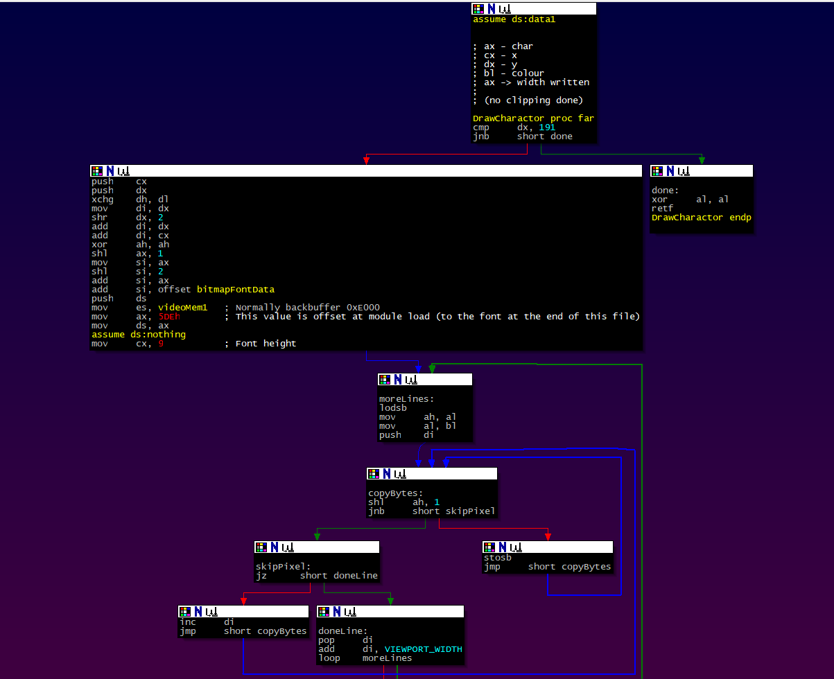
Back in IDA land, it started to become clear I should have been using the graph view for the disassembly all along! The graphical structure really helps give you a mental model of the code - there is not much structure that is quickly visible from a flat assembly listing (unlike indented code), so it's easy to get lost.
At some point in the process, I found the following existing reverse engineering work, this was an immense help both to verify existing work, and to find new jumping off points in the code when I started to run out of steam:
- Jongware - Documents the Frontier Model code in detail for Frontier: First Encounters (FFE). It has a lot of good info, but some missing bits.
- GL Frontier - Frontier running natively on PC using OpenGL. It's done by code converting the AtariST assembly into C, with manual assembly patches to hook into SDL / OpenGL. Has some bugs / limitations, but in general looks really great.
Amiga Blitter
The Amiga has a co-processor called the Blitter, capable of drawing lines and filling spans (i.e. drawing polygons), but FE2 only used it to clear the screen. The Blitter was best suited to working in parallel with the CPU and doing memory intensive operations, to make use of all the available memory bandwidth.
But it was a bit tricky to use the Blitter for rendering polygons, it required a multi-step process for each polygon:
- Clip polygons to screen (CPU)
- Draw polygon outline (edges or curves!) to a temp buffer (CPU or Blitter depending...)
- Composite temp buffer & fill spans to the screen buffer (Blitter)
Each Blitter operation in this process would have to be fed either by via an interrupt or, more likely, from a Copper list. In this case the Copper instructions for each graphics primitive must be written by CPU and then read back & processed by the Blitter. For small polygons this is a lot of overhead, and may not have been worth it.
With the wide variety of graphics primitives rendered, at any point during the render if you have to switch back to using the CPU to render, then you need multiple Copper lists and to manage separate draw lists of stuff for CPU to render / stuff Blitter to render.
Also, even if your Amiga has an upgraded CPU the Blitter still runs at the same speed (the game was developed on an Amiga 2000 with a 68030 accelerator card).
Anyway, in the end for FE2, the CPU was used as the rasteriser. No doubt this was also partly due to having to write CPU rasteriser code for the AtariST anyway and the marginal, if any, performance return on using the Blitter in the given circumstances.
For a discussion on this issue, see: StackExchange - Why Amiga Blitter was not faster than AtariST for 3D
This is not to say the Blitter couldn't be a better option, it's all just engineering trade-offs. It's totally possible you could set things up so that the Blitter is the better option, but that would likely be a very different looking game.
It's worth noting the span renderers are kind of setup in a way that could be used to feed the Blitter, so perhaps that was tried and abandoned. Seems likely it was used in a previous incarnation of the renderer or at least in some experiments.
Music & Sound
The FE2 music is implemented in a custom module format. The custom format has many of the features typical of .mod player: sample list, tracks and sample effects (volume fade, volume changes, vibrato, portamento). There are only about 12 total samples / instruments used by all tracks in the game.
When sound effects are required by the game, they are slotted into free audio channels - or temporarily override an audio channel used by the music if no free audio channel is found. It's surprising how well this works. Most of the time I'm hard-pressed to hear the skipped audio channels in the music track.
All music and sounds can be played by the C remake, you will need to modify the code to hear them though.
On the PC, the sound hardware available was varied. FE2 supported several audio options, from built-in PC Speaker tones to the SoundBlaster card. Music was played directly as MIDI output if the hardware was available. It may sound good on a real Roland HW, but it's a bit chirpy and clipped when listening via DOSBox. I like the Amiga version's sound & music the best, but maybe that's just me.
Module System
This is not part of the 3D engine or even covered by my intro conversion, but the original code has a module system, where different parts of the game are slotted into the main run-loop. Each one is responsible for some part of the game, and has hooks for setup & unload, 2D rendering, 3D rendering, input, and game logic updates. The main game has a big structure for game state and a jump table for game functions, each module can use this to interact with the main game, to query and modify game state, play sounds, render 3D and 2D graphics, etc. The PC version makes use of this to fit into 640K, by only loading parts of the code that are needed e.g. unloading the intro during the main game. It may have been useful during development as well, since compiling the whole game probably took a while given the sheer amount of assembly!
Conclusion
I hope this has given you a feel for the inner workings of the renderer. What's really mind-blowing is that this is just the rendering part. The whole galaxy, game and simulation parts are separate, and likely even more complex.
This post is just a summary of some parts of the renderer - a full description of the code, background and possible considerations that went into it would be immense.
Is there anything you would do differently? What do you think of the colour matching v.s. dithering? Do any modern techniques apply: e.g. vertex ordering for backface culling, subpixel precision?
Further Reading
- Jongware - Documents the Frontier Model code in detail for Frontier: First Encounters (FFE). It has a lot of detailed info about the model code, and how the star systems are generated.
- GL Frontier - Frontier running natively on PC using OpenGL. It's done by auto converting the AtariST assembly into C, with manual assembly patches to hook into SDL / OpenGL. Has some bugs / limitations, but in general looks really great.
- FrontierAstro - Elite / Frontier / FFE info, history and downloads.
- FrontierVerse - Frontier: Elite II info, history and downloads.
- Bézier Rendering
- Amiga Real Time 3D Graphics Book
Acknowledgements
Based on original data and algorithms from "Frontier: Elite 2" and "Frontier: First Encounters" by David Braben & Frontier Developments.
Original copyright holders: